Where did the Binary Cross-Entropy Loss Function come from?

Supplementary part of the blog post “Nothing but NumPy: Understanding & Creating Binary Classification Neural Networks with Computational Graphs from Scratch”

Binary Classification presents a unique problem where:

1. each example (x, y) belongs to one of two complementary classes,
2. each example is independent of each other(i.e result of one example does not affect the outcome of the other example) and,
3. all the examples are generated are from the same underlying distribution/process (i.e if we create a dataset for “cat vs. not-cat” detection then all the examples we feed into the neural network for training “cat vs not-cat” should be from the same dataset and not from a different unrelated dataset such as that for “dog vs. not-dog” ).

In statistics and probability theory attributes 2 and 3 are collectively called i.i.d ( independent and identically distributed). The i.i.d assumption helps to make a lot of the calculations much simpler.

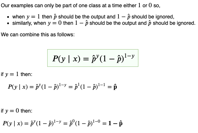
Further, we only need to predict for the positive class i.e P(y=1 | x ) = p̂ because the probability for the negative class can be derived from it i.e P(y=0 | x ) = 1-P(y=1 | x ) = 1-p̂.

A good binary classifier should produce a high value of p̂ when the example has a positive label (y=1). On the other hand, for a negative labeled example (y=0) the classifier should produce a low value of p̂. In other words:

• Maximize p̂ when y=1 and,
• Maximize 1-p̂ when y = 0.

Let’s see how we can combine this intuition into a single expression:

Turns out the single-line expression we came up with, in the above figure, is called a Bernoulli Distribution, and calculating it for a single data point is called a Bernoulli trial. We need to maximize the Bernoulli Distribution for every trial, how do we do that? That’s pretty simple, recall from your high school days that the maximum (or minimum) of any convex function (u-shaped function) occurs at the points where the 1ˢᵗ derivative is equal to zero.

Calculations with the Bernoulli Distribution expression and its derivative can get a bit hairy in its current form, not to mention multiplication and exponentiation of small values can be numerically unstable and can cause a numerical overflow. Luckily the natural logarithm*(represented by “log”, not “ln”)* can help us out here.

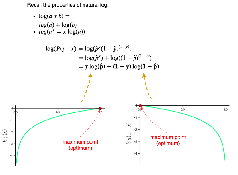
Notice that after applying natural log to the Bernoulli Distribution we have simplified the expression into a sum of log of probabilities. Also, note this simplified expression is awfully similar to the Binary Cross-Entropy Loss function but with the signs reversed. To reach the max point of the log of Bernoulli Distribution through a numerical method (i.e iteratively moving in the direction of the optimum point) we would need to perform “gradient ascent” as the curve of the log function bows upwards (Fig.4), i.e., concave. In neural networks, we prefer to use gradient descent instead of ascent to find the optimum point. We do this because the learning/optimizing of neural networks is posed as a “minimization of loss” problem, so this is where we add the negative sign to the log of Bernoulli Distribution, the result is the Binary Cross-Entropy Loss function:

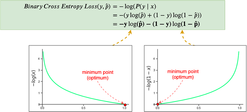
Notice that maximizing the log of Bernoulli Distribution is the same as minimizing the negative log of Bernoulli Distribution. The minimum point and maximum point occur at the same point, now we can easily apply gradient descent and move down the curve to the optimum point.

Using a concept called maximum likelihood estimation (MLE) we can extend the Bernoulli Distribution and come up with the Binary Cross Entropy Cost function. Recall that for a single data point we are maximizing a Bernoulli trial, for multiple data points we will maximize the product of multiple Bernoulli trials.

Consider the following example where we have two classifiers A, and B which give probability predictions on three i.i.d examples:

• Classifier-A : P(X₁), P(X₂), P(X₃) = 0.7, 0.8, 0.9
• Classifier-B : P(X₁), P(X₂), P(X₃) = 0.8, 0.8, 0.8

So which classifier is more likely to be the better classifier for our three examples X₁, X₂ & X₃?

According to MLE the classifier with the highest product of probabilities is likely to be the more superior classifier. Let’s check:

• Classifier-A : P(X₁) × P(X₂) × P(X₃) = 0.7 × 0.8 × 0.9 = 0.504
• Classifier-B : P(X₁) × P(X₂) × P(X₃) = 0.8 × 0.8 × 0.8 = 0.512

So Classifier-B is more likely to be the better classifier.

Applying this concept to multiple independent Bernoulli trials (a distribution with multiple independent Bernoulli trials is called a Binomial distribution) and maximizing the probability for each of the “m” examples in a dataset/batch we get:

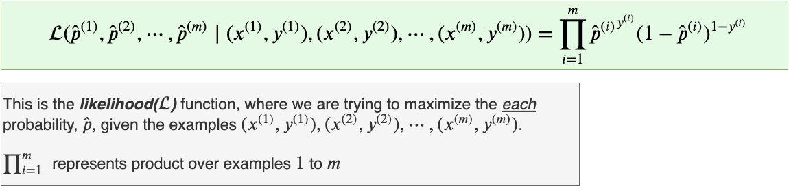
The likelihood function in its current form is prone to numerical overflow because of multiple products. So we will instead take the natural log of the likelihood function.

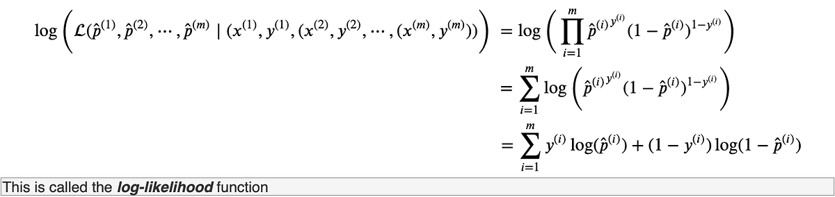
Recall that maximizing a function is the same as minimizing the negative of that function.

Since scaling a function does not change a function’s maximum or minimum point(eg. minimum point of y=x² and y=4x² is at (0,0)), so finally, we’ll divide the negative log-likelihood function by the total number of examples(m) and minimize that function. Turns out it’s the Binary Cross-Entropy(BCE) Cost function that we’ve been using.

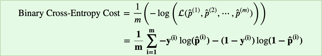
On a final note, our assumption that the underlying data follows as Bernoulli Distribution has allowed us to use MLE and come up with an appropriate Cost function. This assumption/knowledge of data is called a “prior” in Bayesian statistics.

For any questions feel free to reach out to me on Twitter @RafayAK and check out the rest of the post on “binary classification”.